This is the second part of the series on the Taxi Fare prediction problem from an Oracle perspective. You can read Episode 1
here. In this Episode, I will put our model to work. That is, I will show several queries that predict taxi fares based on the features previously selected. I will also review model performance metrics. Remember, performance in this case does not relate to response time, but to fitness or how accurate the predictions are expected to be. Finally, I will comment on the pros and cons of this approach.
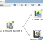 Simple workflow to create GLM and SVM models[/caption] This simple workflow reads the data from the table, obtains basic statistics information of it (Explore data node) and generates a GLM and an SVM model with default parameters (Regress Build 1 node). This workflow can be executed immediately or scheduled to be executed later. This is useful if the base data changes regularly to keep the models trained with the newest data. Once the workflow has been executed we can review each model information and, quite interestingly, a comparison of both models. Like so: [caption id="attachment_105820" align="aligncenter" width="150"]
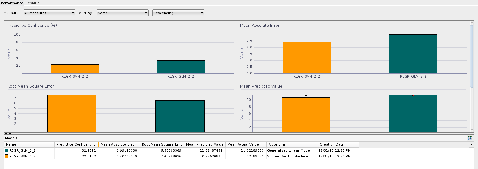
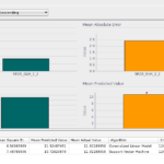 GLM_vs_SVM[/caption] As we can see on the graph, both models perform similarly, but the SVM model shows a slightly worse predictive confidence of 22% compared with the 32% of the GLM model, which is not that good either. This shows that the models do not fit very well for this particular data set. It may be a matter of training with more data or preparing the data in a different way to obtain better results. I may try and add a third episode to this series with attempts at improving the results.
Show me the... results!
Well, now that we have a model what we all want is to see how it fares (see what I did here?). Of course, Oracle includes predictive functions in the Analytics option feature Data Mining SQL Functions. For this exercise, I will use the PREDICTION function because, well, we are predicting stuff. This function has a relatively simple but powerful syntax allowing the introduction of grouping options, cost base data and predictors for regression, classification and anomaly detection problems. It also has two modes of operation: Syntax and Analytic Syntax. Simply put, we can use an existing model with the Syntax option, or we can use the Analytic Syntax option to "create a model on the fly". Let's see a simple example showing both the actual fare amount and the one predicted by the model just for the first 10 rows in the data. First, using the linear regression model created on the 54 million rows train data table we can see that the variation in percentage is quite high, as much as 49% only for this small test set.SQL> WITH PREDICTION AS
2 (SELECT FARE_AMOUNT, PREDICTION (LIN_REG_TAXI_FARE_3 USING *) PREDICTED_FARE
3 FROM TRAIN_DISTANCE_BUCKET_3
4 WHERE CASEID < 11
5 )
6 SELECT FARE_AMOUNT,
7 ROUND(PREDICTED_FARE,2) PREDICTED_FARE,
8 ROUND(ABS(FARE_AMOUNT-PREDICTED_FARE),2) ABS_DIFF,
9 ROUND(ABS(FARE_AMOUNT-PREDICTED_FARE)/FARE_AMOUNT*100,2) "%DIFF"
10 FROM PREDICTION;
FARE_AMOUNT PREDICTED_FARE ABS_DIFF %DIFF
----------- -------------- ---------- ----------
6.5 8.81 2.31 35.48
5.7 8.53 2.83 49.71
10.9 12.25 1.35 12.4
18 18.64 .64 3.54
6.1 7.92 1.82 29.89
13 12.64 .36 2.81
8.5 10.56 2.06 24.2
9 10.99 1.99 22.07
6.5 8.67 2.17 33.36
9.3 10.35 1.05 11.26
10 rows selected.
Elapsed: 00:00:04.275
And now for the support vector machine model created on the 2 million rows train data table. Simply based on these cases, it looks like the SVM model is more accurate that the GLM one.
SQL> WITH PREDICTION AS
  2 (SELECT FARE_AMOUNT, PREDICTION (LIN_REG_TAXI_FARE_3_SVM USING *) PREDICTED_FARE
  3 FROM TRAIN_DISTANCE_BUCKET_3
  4 WHERE CASEID < 11
  5 )
  6 SELECT FARE_AMOUNT,
  7 ROUND(PREDICTED_FARE,2) PREDICTED_FARE,
  8 ROUND(ABS(FARE_AMOUNT-PREDICTED_FARE),2) ABS_DIFF,
  9 ROUND(ABS(FARE_AMOUNT-PREDICTED_FARE)/FARE_AMOUNT*100,2) "%DIFF"
  10 FROM PREDICTION;

 FARE_AMOUNT PREDICTED_FARE ABS_DIFF %DIFF
 ----------- -------------- ---------- ----------
  6.5 7.79 1.29 19.91
  5.7 7.24 1.54 26.96
  10.9 11.99 1.09 10.04
  18 20.4 2.4 13.32
  6.1 6.38 .28 4.58
  13 12.51 .49 3.75
  8.5 9.9 1.4 16.43
  9 9.61 .61 6.73
  6.5 7.31 .81 12.53
  9.3 8.62 .68 7.32

 10 rows selected.

 Elapsed: 00:00:05.736
Another interesting function that Oracle provides is the
PREDICTION_DETAILS function. This function returns an XML string that describes the attributes of the prediction, that is for a prediction problem, the topN attributes that have the most influence in the prediction and their relative weights. Let's see another simple example with the GLM:
SQL> SELECT FARE_AMOUNT,
  ROUND(PREDICTION (LIN_REG_TAXI_FARE_3 USING *),2) PREDICTED_FARE,
  REDICTION_DETAILS (LIN_REG_TAXI_FARE_3 USING *) DETAILS
  FROM TRAIN_DISTANCE_BUCKET
  WHERE CASEID <11;

 FARE_AMOUNT PREDICTED_FARE DETAILS
 ----------- -------------- ------------------------------------------------------------------------------------------
  6.5 8.81
  5.7 8.53

  10.9 12.25

  18 18.64

  6.1 7.92

  13 12.64

  8.5 10.56

  9 10.99

  6.5 8.67

  9.3 10.35

 10 rows selected. Elapsed: 00:00:04.176
Something to note in the example above is that Oracle does not always choose the same attributes and the number of attributes does not seem to imply higher accuracy. But this is only a small portion of the data and may not be representative. Now, the same with the SVM model:
SQL> SELECT FARE_AMOUNT, ROUND(PREDICTION (LIN_REG_TAXI_FARE_3_SVM USING *),2) PREDICTED_FARE,
  2 PREDICTION_DETAILS (LIN_REG_TAXI_FARE_3_SVM USING *) DETAILS
  3 FROM TRAIN_DISTANCE_BUCKET_3
  4 WHERE CASEID <11;

 FARE_AMOUNT PREDICTED_FARE DETAILS
 ----------- -------------- ------------------------------------------------------------------------------------------------------------------------
  6.5 7.79
  5.7 7.24

  10.9 11.99

  18 20.4

  6.1 6.38

  13 12.51

  8.5 9.9

  9 9.61

  6.5 7.31

  9.3 8.62

 10 rows selected. Elapsed: 00:00:04.346
Again, we can see that Oracle is choosing different attributes for each case. In any case, once the model has been created it is quite easy to use SQL, either in batch mode or real time, to obtain predictions.
Model fitness
There are several methods to evaluate the accuracy of a regression model. The Oracle documentation mentions two commonly used: Root Mean Squared Error (RMSE) and Mean Absolute Error (MEA), and provides SQL to calculate them. So let's do it first for the GLM and then for the SVM model.-- First for the GLM model
SQL> with prediction as
2 (SELECT FARE_AMOUNT, PREDICTION (Lin_reg_taxi_fare_3 USING *) PREDICTED_FARE
3 FROM train_distance_bucket_3)
4 select SQRT(AVG((predicted_fare - fare_amount) * (predicted_fare - fare_amount))) rmse,
5 AVG(ABS(predicted_fare - fare_amount)) mae
6* from prediction p;
RMSE MAE
---------- ----------
6.66524393 2.96620921
Elapsed: 00:01:39.752
-- Then for the SVM model
SQL> with prediction as
2 (SELECT FARE_AMOUNT, PREDICTION (LIN_REG_TAXI_FARE_3_SVM USING *) PREDICTED_FARE
3 FROM train_distance_bucket_3 )
4 select SQRT(AVG((predicted_fare - fare_amount) * (predicted_fare - fare_amount))) rmse,
5 AVG(ABS(predicted_fare - fare_amount)) mae
6 from prediction p ;
RMSE MAE
---------- ----------
7.76230946 2.39739187
Elapsed: 00:01:42.077
With the data above we can say that the GLM model is better in general error terms, smaller RMSE. But based on the MAE, the SVM model is slightly better. Note that in the code, both calculations have been performed on the 54 million rows table, although the SVM model was trained with only 2 million rows of data. While Oracle
indicates that the SVM model is more complex and powerful than GLM, for this particular data set it shows worse performance. This may be because the SVM algorithm is better suited to a data set with a large number of attributes, which is not the case here. For those of you who have worked with the original Taxi Fare problem you may know that the RMSE for a basic algorithm is approximately 8, so getting a value of 6.6 is quite an improvement.
Model fitness obtained with the Data Miner
As I explained in Episode 1, the Data Miner extension for SQL*Developer provides tools to create models like the ones I've created with PL/SQL, but based on a GUI used to define what they call a data workflow. In the simplest way to do it, I've created a very simple workflow that starts with the same data table I used to create the first ones, and had the DM to create both a GLM and a SVM regression model with its own default parameters. [caption id="attachment_105819" align="aligncenter" width="150"]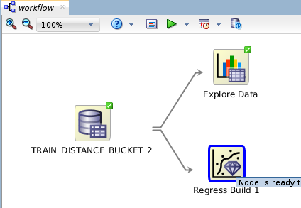 Simple workflow to create GLM and SVM models[/caption] This simple workflow reads the data from the table, obtains basic statistics information of it (Explore data node) and generates a GLM and an SVM model with default parameters (Regress Build 1 node). This workflow can be executed immediately or scheduled to be executed later. This is useful if the base data changes regularly to keep the models trained with the newest data. Once the workflow has been executed we can review each model information and, quite interestingly, a comparison of both models. Like so: [caption id="attachment_105820" align="aligncenter" width="150"]
 GLM_vs_SVM[/caption] As we can see on the graph, both models perform similarly, but the SVM model shows a slightly worse predictive confidence of 22% compared with the 32% of the GLM model, which is not that good either. This shows that the models do not fit very well for this particular data set. It may be a matter of training with more data or preparing the data in a different way to obtain better results. I may try and add a third episode to this series with attempts at improving the results.

