Three Easy Steps For Consolidating Oracle Databases into Cloud Virtual Machines

Karun Dutt

June 20, 2019

Tags: MySQL, Technical Track, Net_Read_Timeout, Wait_Timeout, Net_Write_Timeout, Interactive_Timeout

Problem

Having decided to move our Oracle databases to the cloud, we now want to build equivalent VMs as database servers. This is simple enough when we have only one or a very small number of databases. But this can be a complex task when our environment has multiple Oracle databases. Technologies such as Oracle RAC will further complicate things. Why would we not use the Oracle database as a managed service instead? Short answer: In our case, the cloud vendor of choice does not offer this service, or possibly we are just trying to compare the costs for deciding if managed services are better (they are, but that is another blog post!) Hence, we’ll have questions such as:

How do we estimate our VM footprint for hosting our Oracle databases in the cloud? (Finding the balance between over-provisioning and consolidation.)
How many VMs will we need?
What sizes for vCPU and RAM should we be aiming for?

Of course, we could use a model of deploying one VM per database but this will undoubtedly lead to over-provisioned (virtual) hardware and there may be other factors that affect the practicality or cost; for example, licenses and management of security or monitoring agents, etc. Consequently, we need to look for a cloud VM configuration that allows us to align databases with virtual servers in an optimal manner.

Basic ideas

A "physical" Oracle database server uses three measurable resources:

CPU (to run server and background processes)
Memory - RAM (to cache parts of the database and provide working buffers used by the server and background processes)
Disk (to store and retrieve the data )

For all three dimensions, it is critical to work out what is required and to not just rely on what was previously provisioned. And for the sake of example, we will assume that all databases can coexist and that there are no other non-functional influencers such as departmental billing, security isolation requirements, etc, that would affect or limit the consolidation options. Simple stacking of resources (based on the existing infrastructure) will, of course, lead to an over-provisioned and cost-ineffective cloud solution. AWR, ASH and database settings can give us indicators for a database across a collection period:

CPU used by active sessions as Average Active Sessions (AAS)
RAM allocated (SGA and PGA settings)
Disk
- Throughput Megabytes per second (MBPS)
- IO operations IOPS ( IO per second)
- Filesystem (or ASM) space usage (GB)

An easy starting point is to use AWR and ASH data by running some performance data collection scripts provided by Carlos Sierra and his colleagues ( https://github.com/carlos-sierra/esp_collect ). From that output, we can build a summary table of our databases and their "resource needs". For example, we could have built the table shown below. Note: The databases shown here are fictional -- so YMWV ( your mileage will vary!)

Of course, the obvious caution here is that the metrics are based on ASH and AWR data collected from the Oracle databases. So it’s only as good as the AWR data provided. For an accurate representation of database performance, it may be necessary to adjust your AWR snapshot frequency and/or data retention or to run the analysis process several times with different data collections to ensure an accurate/consistent set of performance metrics to work with.

The Cloud VM as a DB Server

Every cloud VM is also allocated CPUs, RAM and disks, but with a few important differences.

vCPUs are not "full" hyper-threaded CPUs, and we need to provide a conversion factor to convert AAS to vCPUs. After comparing results from www.spec.org, we decided for our purposes (and for our specific cloud provider) that AAS*1.5 = 1 vCPU.
All access to disk is via a network, and network access is limited (max 2GBPS/vCPU in our case).
MBPS and IOPS may be dependent on the type, size of disk and the vCPUS used in the VM.
We will keep a few vCPUs unused to provide for the OS and tools that may be running on the VM.

After reviewing the different constraints, we can come up with a table of "capacities" for each VM type that our cloud provider offers. Some examples: hm-32 Indicates a High Memory VM of 32 vCPUs and 208 GB RAM s-8 is a standard VM of 8 vCPUs and 30 GB RAM The costs of running the VM (for these examples) are calculated for a full 730 hours (a month) with no usage discounts . We are also assuming that we can allocate at most 50% of RAM to the database SGA. Table of Capacities for available VMs shapes:

The Process

We are going to choose the ideal VM sizes that will host all five of our example databases by answering a few questions. Our tools are a Jupyter notebook running Python 3.7 and a sqlite database holding the collected data.

1. What are we are trying to maximize ?

Typically, we want to utilize all the resources that we pay for each month. So each month we want to maximize VMUSAGE where: VMUSAGE = (Cents paid for a VM / Cents wasted ) Cents wasted = Cents paid for - Cents actually Utilized This makes sense. We do not want to pay for vCPUS and RAM that we do not use. But it is still a bit ambivalent. We can get the same VMUSAGE with different sizes of VMs. So how do we get VMUSAGE to be higher for our ideal choice? After a bit of thought, it is clear that we must add "weightage" to larger VMs -- we want to choose the largest VM where we waste the least . Since bigger VMs cost more, let's multiply with the cents we pay for each VM as a weightage. So our (new) VMUSAGE factor that we seek to maximize is VMUSAGE = (Cents paid for a VM) * (Cents paid for a VM / Cents wasted ) If Cents wasted = 0 then set Cents wasted = 0.0001

Note 1: If we are not wasting anything, VMUSAGE will be infinite. So we can put a boundary condition for that in our code. That is the reason for the “if” caveat. Note 2: It does not have to be this way all the time! We could be solving for a VMUSAGE calculated differently. Let's just work with this one for now ... it seems to do the job well enough. So now we are ready for the first VM TYPE and we are evaluating VMUSAGE after we pick databases for it.

2. Given a VM Type, which databases do we choose to put in it?

This is a classical Bin packing problem: see https://developers.google.com/optimization/bin/knapsack to understand this, including some sample Python code blocks that show how to solve this problem using the Google OR-Tools collection of libraries and APIs. However, in our case, we will use the multi-dimensional Solver with the many capacity constraints that our VMs have. Let us call our Solver (in the OR-Tools Knapsack APIs called by the Python block) "DBAllocate": solver = pywrapknapsack_solver.KnapsackSolver( pywrapknapsack_solver.KnapsackSolver.KNAPSACK_MULTIDIMENSION_CBC_MIP_SOLVER, "DBAllocate") The Solver takes three inputs, all of which are arrays:

Value: The "intrinsic value" of picking a specific DB. Since we are trying to maximize resource utilization, this is simply the cents used for running the DB in the VM (again this is a simplification, we could calculate this differently; we could score each DB by its "criticality," for example)
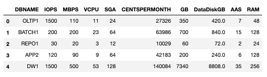
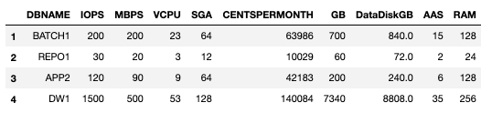
Observations: This is the resources that each DB utilizes from the capacities. We are choosing IOPS, MBPS, VCPU, SGA as the four resources that each DB will use from the VM. This data is sourced from our AWR mining script outputs. Notice we did not include the data disk size which is not affected by the VM type that we select.
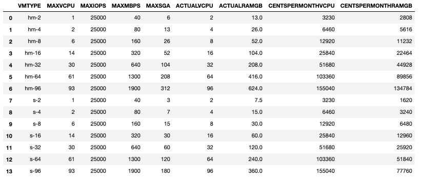
Capacities: The VM has fixed limits for IOPS, MBPS, VCPU, SGA which we will read from our capacities table. The values in the capacities table should been have chosen after allowing for a little bit of overhead for growth and also measurement inaccuracies, so we are using our data engineering experience here.

That done, we call the Solver to do its magic, and can check which are the suggested databases it selects. Sample code lines after defining the three arrays (value, observations, capacities): ## Solve for Capacities and Observations solver.Init(value, observations, capacities) numItemsServed = solver.Solve() ## Check Solution dbsallocated = [x for x in range(0, len(observations[0])) if solver.BestSolutionContains(x)] print(dbsallocated) The dbsallocated array shows the “indexes” of the selected databases, which we can now use to get the rest of the details from the databases table.

3. Rinse/repeat until we allocate all databases

First Iteration

We are allowing the Knapsack Solver to pick the databases for us for all VM types and then calculate VMUSAGE for the database selection for each VM Type. The Solver goes through all of the possible permutations to find the optimal configuration. The VMUSAGE shows up very different values for all VM types, higher numbers are better! VMs that cannot accommodate any databases are showing a VMUSAGE of 0.

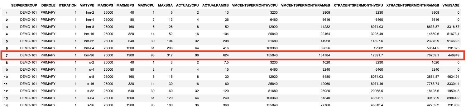
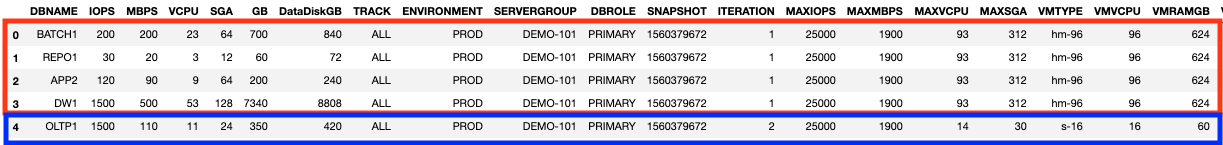
For Iteration 1 the highest VMUSAGE is for a VM of type: hm-96 (Row 7) The Solver determines that the VM hm-96 will contain the following databases (it has used 88 of the available 93 vCPUs).

Second Iteration

After we remove the databases already selected in the first Iteration, we are left with only 1 database to allocate! The code runs the second iteration automatically as long as there are databases yet to be allocated. Re-running the VMUSAGE calculation to find the best VM to hold the last remaining database

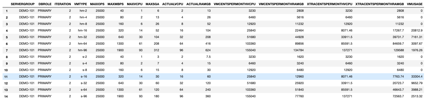
The highest value for VMUSAGE is for VM type S-16 (Row 11). So we have a complete solution in two iterations.

The Solution

In our example, we can do a dense packing of our five databases in two kinds of VMs to minimize expected costs. The VM type hm-96 hosts the first four databases (BATCH1, REPO1, APP2, DW1) and the VM type s-16 hosts one database (OLTP1).

Strong disclaimer: The costs used in the capacities table are an estimate for each of the VM types and are focused on vCPU and RAM . For an actual server, there will be additional expenses for network, disks for the databases, backups etc. which we can factor in as well, but we have kept it simple. There may also be additional savings based on commitments, sustained usage discounts, etc . The cents per month are used to choose VMs for optimization and do not reflect actual costs!

Conclusion & Acknowledgements

With a few simplifying assumptions we can model our requirements as a use-case of the well known multi-dimensional Knapsack problem. Using the Google OR-Tools toolkit, data mined from the Oracle AWR and ASH, and some simple Python code, we can develop a future-state configuration based on our cloud provider’s VM shapes. We used AWR and ASH metrics collected using the publicly available esp-collection framework courtesy of Carlos Sierra and his colleagues ( https://github.com/carlos-sierra/esp_collect ). Google OR-Tools gave us the Knapsack Solver API ( https://developers.google.com/optimization/bin/knapsack ) and the starting Python code that we built on. Let me know in your comments if you have any suggestions and your experiences!

Code

SQL Code to be used to create database tables

[sourcecode language="sql" wraplines="false" collapse="true"] ############# tables for Solver ########## ## ## table: vmconfig ## drop table vmconfig; create table vmconfig( VMTYPE varchar(100), MAXVCPU NUMERIC, MAXIOPS NUMERIC, MAXMBPS NUMERIC, MAXSGA NUMERIC, ACTUALVCPU NUMERIC, ACTUALRAMGB NUMERIC, CENTSPERMONTHVCPU NUMERIC, CENTSPERMONTHRAMGB NUMERIC ); begin transaction; insert into vmconfig values('hm-2',1,25000,40,6,2,13,0,0); insert into vmconfig values('hm-4',2,25000,80,13,4,26,0,0); insert into vmconfig values('hm-8',6,25000,160,26,8,52,0,0); insert into vmconfig values('hm-16',14,25000,320,52,16,104,0,0); insert into vmconfig values('hm-32',30,25000,640,104,32,208,0,0); insert into vmconfig values('hm-64',61,25000,1300,208,64,416,0,0); insert into vmconfig values('hm-96',93,25000,1900,312,96,624,0,0); insert into vmconfig values('s-2',1,25000,40,3,2,7.5,0,0); insert into vmconfig values('s-4',2,25000,80,7,4,15,0,0); insert into vmconfig values('s-8',6,25000,160,15,8,30,0,0); insert into vmconfig values('s-16',14,25000,320,30,16,60,0,0); insert into vmconfig values('s-32',30,25000,640,60,32,120,0,0); insert into vmconfig values('s-64',61,25000,1300,120,64,240,0,0); insert into vmconfig values('s-96',93,25000,1900,180,96,360,0,0); commit; ## ## table: dbdetails ## drop table dbdetails; create table dbdetails( DBNAME varchar(100), AAS NUMERIC, SGA NUMERIC, MBPS NUMERIC, IOPS NUMERIC, GB NUMERIC, CENTSPERMONTH NUMERIC ); begin transaction; insert into dbdetails values('OLTP1',7,24,110,1500,350,0); insert into dbdetails values('BATCH1',15,64,200,200,700,0); insert into dbdetails values('REPO1',2,12,20,30,60,0); insert into dbdetails values('APP2',6,64,90,120,200,0); insert into dbdetails values('DW1',35,128,500,1500,7340,0); commit; ############ END ################################################### [/sourcecode]

Python Code to be used in the Notebook

[sourcecode language="python" wraplines="false" collapse="true"] #!/usr/bin/env python # coding: utf-8 ## Uncomment to Run once when we start the Notebook to install dependencies ## !pip install pandas ##!pip install matplotlib ##!pip install -U ortools # Will allow us to embed Plots in the notebook get_ipython().run_line_magic('matplotlib', 'inline') from __future__ import print_function import datetime import sqlite3 import pandas as pd import numpy as np import matplotlib.pyplot as plt import time ## Importing OR tools Knapsack Solver from ortools.algorithms import pywrapknapsack_solver ## Choose DB Directory path and data area escpdirectory = '~/db' sqlitedbname = 'solver.db' snapshot_retain='Y' snapshotN = int(datetime.datetime.now().strftime('%s') ) print ('Starting timestamp: %d' %snapshotN) iteration=0 ## Enter the charges for vCPU and RAM GB per month in Cents chargecentspermonthvcpu=1615.3221 chargecentspermonthramgb=216.5107 # Create the connection to Master DB cnx = sqlite3.connect(r'%s/%s' %(escpdirectory, sqlitedbname)) ## Update the charges on the VMConfig and DB details ## We are assuming ## AAS = 1.5 vCPU ## RAM needed = 2 * SGA cur = cnx.cursor() cur.execute('begin transaction') cur.execute('''update vmconfig set CENTSPERMONTHVCPU = ACTUALVCPU * %d, CENTSPERMONTHRAMGB = ACTUALRAMGB * %d ''' % (chargecentspermonthvcpu, chargecentspermonthramgb)) cur.execute('''update dbdetails set CENTSPERMONTH = (AAS * 1.5 * %d) + (SGA * 2 * %d) ''' % (chargecentspermonthvcpu, chargecentspermonthramgb)) cur.execute('commit') cur.close() dfvm = pd.read_sql_query(''' select vmconfig.VMTYPE as VMTYPE, vmconfig.MAXVCPU as MAXVCPU, vmconfig.MAXIOPS as MAXIOPS, vmconfig.MAXMBPS as MAXMBPS, vmconfig.MAXSGA as MAXSGA, vmconfig.ACTUALVCPU as ACTUALVCPU, vmconfig.ACTUALRAMGB as ACTUALRAMGB, vmconfig.CENTSPERMONTHVCPU as CENTSPERMONTHVCPU, vmconfig.CENTSPERMONTHRAMGB as CENTSPERMONTHRAMGB from vmconfig ''' , cnx) ##display(dfvm) df = pd.read_sql_query(''' select dbdetails.DBNAME as DBNAME, dbdetails.IOPS as IOPS, dbdetails.MBPS as MBPS, cast (round(dbdetails.AAS * 1.5) as INTEGER) as VCPU, dbdetails.SGA as SGA, cast (round(dbdetails.CENTSPERMONTH) as INTEGER) as CENTSPERMONTH, dbdetails.GB as GB, round(dbdetails.GB*1.2) as DataDiskGB, dbdetails.AAS as AAS, dbdetails.SGA * 2 as RAM from dbdetails ''' , cnx) ##display(df) # Create the solver. solver = pywrapknapsack_solver.KnapsackSolver( pywrapknapsack_solver.KnapsackSolver.KNAPSACK_MULTIDIMENSION_CBC_MIP_SOLVER, 'DBAllocate') dfv=df.copy() print ('To allocate : %d databases' % len(dfv)) display(dfv) track = "ALL" environment = "PROD" servergroup="DEMO-101" dbrole = "PRIMARY" iteration = 0 ## Create the Dataframes to work with the Solver and to hold Retained Solutions dfr = pd.DataFrame(columns=['DBNAME','IOPS','MBPS','VCPU','SGA','GB','DataDiskGB','TRACK', 'ENVIRONMENT','SERVERGROUP', 'DBROLE', 'SNAPSHOT','ITERATION', 'MAXIOPS','MAXMBPS','MAXVCPU','MAXSGA', 'VMTYPE', 'VMVCPU', 'VMRAMGB', 'VMCENTSPERMONTH']) # We build the Iterations that are least wasteful and store them in All Iterations Table as well dfall = pd.DataFrame(columns=['SERVERGROUP','DBROLE','ITERATION','VMTYPE','MAXIOPS','MAXMBPS','MAXVCPU','MAXSGA','ACTUALVCPU','ACTUALRAMGB','VMCENTSPERMONTHVCPU','VMCENTSPERMONTHRAMGB','XTRACENTSPERMONTHVCPU','XTRACENTSPERMONTHRAMGB', 'VMUSAGE']) print('working on : %s - %s' % (servergroup, dbrole)) snapshotN = snapshotN + 20 snapshot = str(snapshotN) ##print(snapshot) while len(dfv) > 0: dfallit = pd.DataFrame(columns=['SERVERGROUP','DBROLE','ITERATION','VMTYPE','MAXIOPS','MAXMBPS','MAXVCPU','MAXSGA','ACTUALVCPU','ACTUALRAMGB','VMCENTSPERMONTHVCPU','VMCENTSPERMONTHRAMGB','XTRACENTSPERMONTHVCPU','XTRACENTSPERMONTHRAMGB', 'VMUSAGE']) ## Start with Current iteration + 1 and find the Highest Utilization iteration = iteration + 1 dfvm = pd.read_sql_query(''' select vmconfig.VMTYPE as VMTYPE, vmconfig.MAXVCPU as MAXVCPU, vmconfig.MAXIOPS as MAXIOPS, vmconfig.MAXMBPS as MAXMBPS, vmconfig.MAXSGA as MAXSGA, vmconfig.ACTUALVCPU as ACTUALVCPU, vmconfig.ACTUALRAMGB as ACTUALRAMGB, vmconfig.CENTSPERMONTHVCPU as CENTSPERMONTHVCPU, vmconfig.CENTSPERMONTHRAMGB as CENTSPERMONTHRAMGB, %d as ITERATION from vmconfig ''' % iteration , cnx) ##display(dfvm) for index, row in dfvm.iterrows(): vmtype = row['VMTYPE'] maxiops = row['MAXIOPS'] maxmbps = row['MAXMBPS'] maxvcpu = row['MAXVCPU'] maxsga = row['MAXSGA'] actualvcpu = row['ACTUALVCPU'] actualramgb = row['ACTUALRAMGB'] iteration = row['ITERATION'] vmcentspermonthvcpu = row['CENTSPERMONTHVCPU'] vmcentspermonthramgb = row['CENTSPERMONTHRAMGB'] capacities = [maxiops, maxmbps, maxvcpu, maxsga] ##print(vmtype, capacities) v = dfv.to_numpy(copy=True).transpose() dbnames=v[0].tolist() observations=np.array([i for i in v[1:5]], dtype=np.int32).tolist() gb=np.array(v[5], dtype=np.int32).tolist() ##print (servergroup, dbrole, iteration, vmtype, dbnames) ## Solve for Capacities and Observations solver.Init(gb, observations, capacities) numItemsServed = solver.Solve() ## Check Solution dbsallocated = [x for x in range(0, len(observations[0])) if solver.BestSolutionContains(x)] ##print(dbsallocated) dfselected=dfv.iloc[dbsallocated ] ##display(dfselected) ## Calculate Usage of Cents and Extra Capacities for the Selected databases in this vmtype totalvcpu = dfselected['VCPU'].sum() totalramgb = dfselected['SGA'].sum() xtracentspermonthvcpu = vmcentspermonthvcpu - (totalvcpu * chargecentspermonthvcpu) xtracentspermonthramgb = vmcentspermonthramgb - (totalramgb * chargecentspermonthramgb) xtracents = xtracentspermonthvcpu + xtracentspermonthramgb actualcents = (totalvcpu * chargecentspermonthvcpu) + (totalramgb * chargecentspermonthramgb) vmcents = vmcentspermonthvcpu + vmcentspermonthramgb ##print('Vmtype : %s Total Cents/Mnth: %d VCPUCents/Mnth : %d RAMCents/Mnth : %d' %(vmtype,vmcents, vmcentspermonthvcpu, vmcentspermonthramgb )) if xtracents > 0 : xtracents = xtracents ##Unchanged else: xtracents = 0.0001 ## To have a Non-zero denominator ##vmusage = efficiency * (totalvcpu * chargecentspermonthvcpu + totalramgb * chargecentspermonthramgb) vmusage = actualcents * actualcents/xtracents ## Append into All Temporary Iterations dataframe lendfallit=len(dfallit) dfallit.at[lendfallit + 1 ,'SERVERGROUP' ] = servergroup dfallit.at[lendfallit + 1 ,'DBROLE' ] = dbrole dfallit.at[lendfallit + 1 ,'ITERATION' ] = iteration dfallit.at[lendfallit + 1 ,'VMTYPE' ] = vmtype dfallit.at[lendfallit + 1 ,'MAXIOPS'] = maxiops dfallit.at[lendfallit + 1 ,'MAXMBPS'] = maxmbps dfallit.at[lendfallit + 1 ,'MAXVCPU'] = maxvcpu dfallit.at[lendfallit + 1 ,'MAXSGA'] = maxsga dfallit.at[lendfallit + 1 ,'ACTUALVCPU'] = actualvcpu dfallit.at[lendfallit + 1 ,'ACTUALRAMGB'] = actualramgb dfallit.at[lendfallit + 1 ,'VMCENTSPERMONTHVCPU' ] = vmcentspermonthvcpu dfallit.at[lendfallit + 1 ,'VMCENTSPERMONTHRAMGB' ] = vmcentspermonthramgb dfallit.at[lendfallit + 1 ,'XTRACENTSPERMONTHVCPU' ] = xtracentspermonthvcpu dfallit.at[lendfallit + 1 ,'XTRACENTSPERMONTHRAMGB' ] = xtracentspermonthramgb dfallit.at[lendfallit + 1 ,'VMUSAGE' ] = vmusage ## End of For Loop dfvm.iterrows ## Extract the Row from the Temporary data frame with max usage and insert it into Chosen Iterations dataframe display(dfallit) maxindex=dfallit['VMUSAGE'].astype('float64').idxmax() lendfall=len(dfall) dfall.at[lendfall+1,'SERVERGROUP'] = dfallit.at[maxindex, 'SERVERGROUP'] dfall.at[lendfall+1,'DBROLE'] = dfallit.at[maxindex, 'DBROLE'] dfall.at[lendfall+1,'ITERATION'] = dfallit.at[maxindex, 'ITERATION'] dfall.at[lendfall+1,'VMTYPE'] = dfallit.at[maxindex, 'VMTYPE'] dfall.at[lendfall+1 ,'MAXIOPS'] = dfallit.at[maxindex, 'MAXIOPS'] dfall.at[lendfall+1 ,'MAXMBPS'] = dfallit.at[maxindex, 'MAXMBPS'] dfall.at[lendfall+1 ,'MAXVCPU'] = dfallit.at[maxindex, 'MAXVCPU'] dfall.at[lendfall+1 ,'MAXSGA'] = dfallit.at[maxindex, 'MAXSGA'] dfall.at[lendfall+1 ,'ACTUALVCPU'] = dfallit.at[maxindex, 'ACTUALVCPU'] dfall.at[lendfall+1 ,'ACTUALRAMGB'] = dfallit.at[maxindex, 'ACTUALRAMGB'] dfall.at[lendfall+1,'VMCENTSPERMONTHVCPU'] = dfallit.at[maxindex, 'VMCENTSPERMONTHVCPU'] dfall.at[lendfall+1,'VMCENTSPERMONTHRAMGB'] = dfallit.at[maxindex, 'VMCENTSPERMONTHRAMGB'] dfall.at[lendfall+1,'XTRACENTSPERMONTHVCPU'] = dfallit.at[maxindex, 'XTRACENTSPERMONTHVCPU'] dfall.at[lendfall+1,'XTRACENTSPERMONTHRAMGB']= dfallit.at[maxindex, 'XTRACENTSPERMONTHRAMGB'] dfall.at[lendfall+1,'VMUSAGE'] = dfallit.at[maxindex, 'VMUSAGE'] ## Remake variables to point to the Chosen Row (rather than the last one) servergroup = dfallit.at[maxindex, 'SERVERGROUP'] dbrole = dfallit.at[maxindex, 'DBROLE'] vmtype = dfallit.at[maxindex, 'VMTYPE'] maxiops = dfallit.at[maxindex, 'MAXIOPS'] maxmpbs = dfallit.at[maxindex, 'MAXMBPS'] maxvcpu = dfallit.at[maxindex, 'MAXVCPU'] maxsga = dfallit.at[maxindex, 'MAXSGA'] actualvcpu = dfallit.at[maxindex, 'ACTUALVCPU'] actualramgb = dfallit.at[maxindex, 'ACTUALRAMGB'] vmcentspermonthvcpu = dfallit.at[maxindex, 'VMCENTSPERMONTHVCPU'] vmcentspermonthramgb = dfallit.at[maxindex, 'VMCENTSPERMONTHRAMGB'] ## Re-run the Vm Type with Max Usage and Remove the Selected databases capacities = [maxiops, maxmbps, maxvcpu, maxsga] ##print(capacities) v = dfv.to_numpy(copy=True).transpose() dbnames=v[0].tolist() observations=np.array([i for i in v[1:5]], dtype=np.int32).tolist() gb=np.array(v[5], dtype=np.int32).tolist() print (' Allocate for ', servergroup, dbrole, iteration, vmtype, dbnames) ## Solve for Capacities and Observations solver.Init(gb, observations, capacities) numItemsServed = solver.Solve() ## Check Solution dbsallocated = [x for x in range(0, len(observations[0])) if solver.BestSolutionContains(x)] ##print(dbsallocated) dfselected=dfv.iloc[dbsallocated ] display(dfselected) ## Update Retained dataframe lendfr=len(dfr) for i in range (0, len(dbsallocated)): dfr.at[lendfr+i,'DBNAME' ] = dfv.at[dbsallocated[i], 'DBNAME'] dfr.at[lendfr+i,'IOPS' ] = dfv.at[dbsallocated[i], 'IOPS'] dfr.at[lendfr+i,'MBPS' ] = dfv.at[dbsallocated[i], 'MBPS'] dfr.at[lendfr+i,'VCPU' ] = dfv.at[dbsallocated[i], 'VCPU'] dfr.at[lendfr+i,'SGA' ] = dfv.at[dbsallocated[i], 'SGA'] dfr.at[lendfr+i,'GB' ] = dfv.at[dbsallocated[i], 'GB'] dfr.at[lendfr+i,'DataDiskGB' ] = dfv.at[dbsallocated[i], 'DataDiskGB'] dfr.at[lendfr+i,'TRACK'] = track dfr.at[lendfr+i,'ENVIRONMENT'] = environment dfr.at[lendfr+i,'SERVERGROUP'] = servergroup dfr.at[lendfr+i,'DBROLE'] = dbrole dfr.at[lendfr+i

Insight and analysis of technology and business strategy