Machine Learning is all about striking the right balance between optimization and generalization. Optimization means tuning your model to squeeze out every bit of performance from it. Generalization refers to making your model generic enough so that it can perform well on the unseen data. As you can see, optimization and generalization are correlated.
When the model is still training and the network hasn’t yet modeled all the patterns, you’ll naturally get lower loss on training (and this results in lower loss on test data). This is called “underfitting.” But after few training iterations, generalization stops improving. As a result, the model starts to learn patterns to fit the training data. This is called “overfitting.” Overfitting is not particularly useful, because your model won’t perform well on the unseen new data.
So, how do we avoid overfitting? Here are few techniques.
Get More Training Data
One way to solve this problem is to have an infinite amount of training data (or at least more training data). More training data translates into the better generalization of your model. But getting more training data is not always possible, because sometimes you’d have to work with the dataset that you have. In this case, it might make sense to only focus on the key patterns that will give you right overall generalization.
Reducing the Network Size
The simplest way to avoid overfitting is to reduce the size of your model. That is, the number of layers or nodes per layer. This is also known as model capacity. In theory, the more capacity, the more learning power for the model. However, the model will train to overfit too well to the training data. So, more powerful models don’t really translate into better generalization and hence better performance. Unfortunately there is no magic formula to determine the number of layers and nodes in your model. You’d have to evaluate your various model architectures in order to size it them correctly.
Here, we’ll be working with the IMDB dataset for movies. Let’s prepare the data.
from keras.datasets import imdb
import numpy as np

(train_data, train_labels), (test_data, test_labels) = imdb.load_data(num_words=10000)

def vectorize_sequences(sequences, dimension=10000):
    # Padding
    results = np.zeros((len(sequences), dimension))
    for i, sequence in enumerate(sequences):
        results[i, sequence] = 1.
    return results

# vectorized training data
x_train = vectorize_sequences(train_data)
# vectorized test data
x_test = vectorize_sequences(test_data)
# vectorized labels
y_train = np.asarray(train_labels).astype('float32')
y_test = np.asarray(test_labels).astype('float32')
To demonstrate this, let’s create two models of different sizes.
Here is the bigger model:
from keras import models
from keras import layers
bigger_model = models.Sequential()
bigger_model.add(layers.Dense(16, activation='relu', input_shape=(10000,)))
bigger_model.add(layers.Dense(16, activation='relu'))
bigger_model.add(layers.Dense(1, activation='sigmoid'))
bigger_model.compile(optimizer='rmsprop',
loss='binary_crossentropy',
metrics=['acc'])
Here is the smaller one:
smaller_model = models.Sequential()
smaller_model.add(layers.Dense(4, activation='relu', input_shape=(10000,)))
smaller_model.add(layers.Dense(4, activation='relu'))
smaller_model.add(layers.Dense(1, activation='sigmoid'))
smaller_model.compile(optimizer='rmsprop',
                      loss='binary_crossentropy',
                      metrics=['acc'])
Now, let’s calculate the validation losses for bigger and smaller networks:
bigger_hist = bigger_model.fit(x_train, y_train,
                                   epochs=20,
                                   batch_size=512,
                                   validation_data=(x_test, y_test))
smaller_hist = smaller_model.fit(x_train, y_train,
                                   epochs=20,
                                   batch_size=512,
                                   validation_data=(x_test, y_test))
Now, let’s plot it:
import matplotlib.pyplot as plt
epochs = range(1, 21)
bigger_val_loss = bigger_hist.history['val_loss']
smaller_val_loss = smaller_hist.history['val_loss']
plt.plot(epochs, bigger_val_loss, 'b+', label='bigger model')
plt.plot(epochs, smaller_val_loss, 'bo', label='Smaller model')
plt.xlabel('Epochs')
plt.ylabel('Validation loss')
plt.legend()
plt.show()
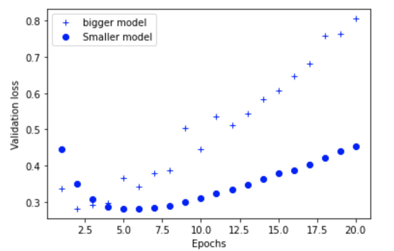
As you can see, the bigger model starts overfitting much faster than the smaller model. The validation loss increases substantially after eight epochs or so.
Now, to take this a bit further, let’s create a model with a much bigger capacity and compare it against the “bigger” model above. Let’s call this new model, “much bigger model.”
much_bigger_model = models.Sequential()
much_bigger_model.add(layers.Dense(512, activation='relu', input_shape=(10000,)))
much_bigger_model.add(layers.Dense(512, activation='relu'))
much_bigger_model.add(layers.Dense(1, activation='sigmoid'))
much_bigger_model.compile(optimizer='rmsprop',
                     loss='binary_crossentropy',
                     metrics=['acc'])
much_bigger_model_hist = much_bigger_model.fit(x_train, y_train,
                                     epochs=20,
                                     batch_size=512,
                                     validation_data=(x_test, y_test))
Now, we compare:
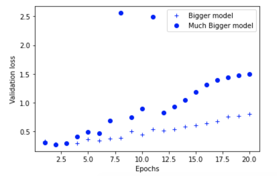
As you can see, the “much bigger model” network starts overfitting almost immediately.
Let’s compare the training losses:
bigger_train_loss = bigger_hist.history['loss']
much_bigger_model_train_loss = much_bigger_model_hist.history['loss']
plt.plot(epochs, bigger_train_loss, 'b+', label='Bigger model')
plt.plot(epochs, much_bigger_model_train_loss, 'bo', label='Much Bigger model')
plt.xlabel('Epochs')
plt.ylabel('Training loss')
plt.legend()
plt.show()
Here is the plot:
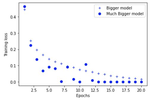
The bigger the network, the sooner it approaches the training loss of zero. In other words, more capacity translates into overfitting the training data.
Regularization
As we saw above, simpler models tend to overfit less than the complex ones. A “simple model” in this case is the one with less overall parameters and hence less value entropy across the board. You can mitigate this by adjusting the distribution of weights, or, in other words, regularizing them. This is typically done by adding loss functions to the network. There are two types:
- L1 regularization: The cost added is proportional to the absolute value of the weight’s coefficients.
- L2 regularization: The cost added is proportional to the square of the value of the weight’s coefficients.
This is the parameter in Keras, as shown below:
from keras import regularizers

l2_model = models.Sequential()
l2_model.add(layers.Dense(16, kernel_regularizer=regularizers.l2(0.001),
                          activation='relu', input_shape=(10000,)))
l2_model.add(layers.Dense(16, kernel_regularizer=regularizers.l2(0.001),
                          activation='relu'))
l2_model.add(layers.Dense(1, activation='sigmoid'))
l2_model.compile(optimizer='rmsprop',
                 loss='binary_crossentropy',
                 metrics=['acc'])
Let’s see how this performs:
l2_model_hist = l2_model.fit(x_train, y_train,
                             epochs=20,
                             batch_size=512,
                             validation_data=(x_test, y_test))
Here is the plot:
l2_model_val_loss = l2_model_hist.history['val_loss']
plt.plot(epochs, bigger_val_loss, 'b+', label='Bigger model')
plt.plot(epochs, l2_model_val_loss, 'bo', label='L2-regularized model')
plt.xlabel('Epochs')
plt.ylabel('Validation loss')
plt.legend()
plt.show()
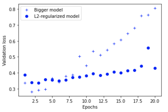
As you can see, the model with L2 regularization is less prone to overfitting compared to the bigger model.
Adding Dropout
Dropout is considered as one of the most effective regularization methods. Dropout is basically randomly zero-ing or dropping out features from your layer during the training process, or introducing some noise in the samples. The key thing to note is that this is only applied at training time. At test time, no values are dropped out. Instead, they are scaled. The typical dropout rate is between 0.2 to 0.5.
In Keras, you can add a dropout to a Dropout layer just after the intended layer, as shown below:
model.add(layers.Dropout(0.5))
drop_model = models.Sequential()
drop_model.add(layers.Dense(16, activation='relu', input_shape=(10000,)))
drop_model.add(layers.Dropout(0.5))
drop_model.add(layers.Dense(16, activation='relu'))
drop_model.add(layers.Dropout(0.5))
drop_model.add(layers.Dense(1, activation='sigmoid'))
drop_model.compile(optimizer='rmsprop',
                  loss='binary_crossentropy',
                  metrics=['acc'])
Now, let’s plot.
drop_model_val_loss = drop_model_hist.history['val_loss']

plt.plot(epochs, bigger_val_loss, 'b+', label='Original model')
plt.plot(epochs, drop_model_val_loss, 'bo', label='Dropout-regularized model')
plt.xlabel('Epochs')
plt.ylabel('Validation loss')
plt.legend()
plt.show()
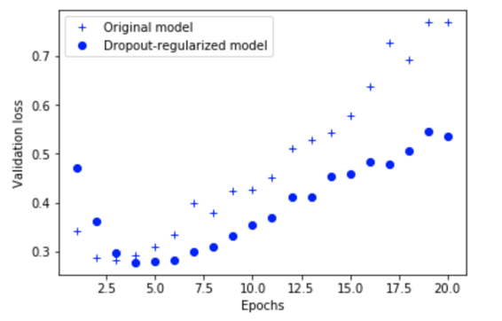
This is much better!
Summary
The most effective way to prevent overfitting in deep learning networks is by:
- Gaining access to more training data.
- Making the network simple, or tuning the capacity of the network (the more capacity than required leads to a higher chance of overfitting).
- Regularization.
- Adding dropouts.
Happy learning!

