 Heart disease covers a range of different conditions that could affect your heart. It is one of the most complex diseases to predict given the number of potential factors in your body that can lead to it. Identifying and predicting heart disease poses a great deal of challenge for doctors and researchers alike. I will attempt to take a stab at this problem using machine learning (ML) with the public dataset available
here at UCI Machine Learning Repository. Let’s get started. There are 303 records in the dataset and it contains 14 continuous attributes. The goal is to predict the presence of heart disease in the patient. The dataset contained an original set of 76 attributes which has now been narrowed down to total of 14 as follows:
age: The person’s age in years
sex: The person’s sex (1 = male, 0 = female)
cp: The chest pain experienced (value 1: typical angina, value 2: atypical angina, value 3: non-anginal pain, value 4: asymptomatic)
trestbps: The person’s resting blood pressure
chol: The person’s cholesterol measurement in mg/dl
fbs: The person’s fasting blood sugar (> 120 mg/dl, 1 = true; 0 = false)
restecg: Resting electrocardiographic measurement (0 = normal, 1 = having ST-T wave abnormality, 2 = showing probable or definite left ventricular hypertrophy by Estes’ criteria)
thalach: The person’s maximum heart rate achieved
exang: Exercise induced angina (1 = yes; 0 = no)
oldpeak: ST depression induced by exercise relative to rest (‘ST’ relates to positions on the ECG plot)
slope: The slope of the peak exercise ST segment (value 1: upsloping, value 2: flat, value 3: downsloping)
ca: The number of major vessels (0 – 3)
thal: A blood disorder called thalassemia (3 = normal; 6 = fixed defect; 7 = reversable defect)
target: Heart disease (0 = no, 1 = yes)
Heart disease covers a range of different conditions that could affect your heart. It is one of the most complex diseases to predict given the number of potential factors in your body that can lead to it. Identifying and predicting heart disease poses a great deal of challenge for doctors and researchers alike. I will attempt to take a stab at this problem using machine learning (ML) with the public dataset available
here at UCI Machine Learning Repository. Let’s get started. There are 303 records in the dataset and it contains 14 continuous attributes. The goal is to predict the presence of heart disease in the patient. The dataset contained an original set of 76 attributes which has now been narrowed down to total of 14 as follows:
age: The person’s age in years
sex: The person’s sex (1 = male, 0 = female)
cp: The chest pain experienced (value 1: typical angina, value 2: atypical angina, value 3: non-anginal pain, value 4: asymptomatic)
trestbps: The person’s resting blood pressure
chol: The person’s cholesterol measurement in mg/dl
fbs: The person’s fasting blood sugar (> 120 mg/dl, 1 = true; 0 = false)
restecg: Resting electrocardiographic measurement (0 = normal, 1 = having ST-T wave abnormality, 2 = showing probable or definite left ventricular hypertrophy by Estes’ criteria)
thalach: The person’s maximum heart rate achieved
exang: Exercise induced angina (1 = yes; 0 = no)
oldpeak: ST depression induced by exercise relative to rest (‘ST’ relates to positions on the ECG plot)
slope: The slope of the peak exercise ST segment (value 1: upsloping, value 2: flat, value 3: downsloping)
ca: The number of major vessels (0 – 3)
thal: A blood disorder called thalassemia (3 = normal; 6 = fixed defect; 7 = reversable defect)
target: Heart disease (0 = no, 1 = yes)
Exploratory Analysis
Before we start the detailed data analysis, let's begin with the exploratory analysis to understand how data is distributed and extract the preliminary knowledge. First things first, download the data from the link provided above and import the dataset to pandas DataFrame. Download the csv file from the link provided above and upload the csv dataset file.
from google.colab import files
 uploaded = files.upload()
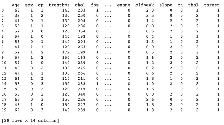
Import the dataset to a pandas DataFrame and print the first 20 records.
import io
 Data = pd.read_csv(io.BytesIO(uploaded['heart.csv']))
 print(Data.head(20))
 With the data imported successfully, let’s plot the distribution between heart disease and the absence of it, indicated by the target attribute.
f = sns.countplot(x='target', data=Data)
 f.set_title("Heart disease distribution")
 f.set_xticklabels(['No Heart disease', 'Heart Disease'])
 plt.xlabel("");
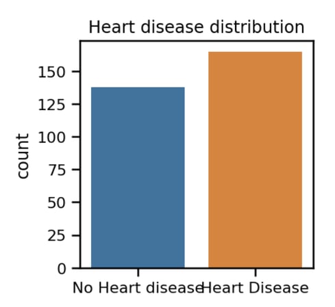 We can see from the above chart that distribution between positive and negative heart disease is almost the same. A good setup for a binary classification ML problem. Next let’s extend above distribution for male and female gender:
f = sns.countplot(x='target', data=Data, hue='sex')
 plt.legend(['Female', 'Male'])
 f.set_title("Heart disease by gender")
 f.set_xticklabels(['No Heart disease', 'Heart Disease'])
 plt.xlabel("");
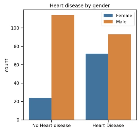 From the above chart we can see that the distribution of "no heart disease" between males and females is skewed. We aren't sure at this point what impact this will have in the final model, if any, or the relationship between the two at this stage. Understanding the relations between various factors that impact on the final outcome of heart disease is a key to this analysis. At this point we've tried to identify the pattern by plotting the individual plots between different factors. There is an alternative way of doing this: correlation matrix or heat map. It is very useful to highlight the most correlated variables in a data table. In this plot, correlation coefficients are coloured according to the value. Let’s plot a heatmap of correlation matrix as below:
heat_map = sns.heatmap(Data.corr(method='pearson'), annot=True,
 fmt='.2f', linewidths=2)
 heat_map.set_xticklabels(heat_map.get_xticklabels(), rotation=45);
 plt.rcParams["figure.figsize"] = (50,50)
[caption id="attachment_108840" align="aligncenter" width="500"]
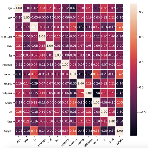 Heatmap between all 14 attributes[/caption] As you can observe there is no strong correlation between any of the 14 attributes.
Building Keras Binary Classifier
After data exploration, it's time to build a Keras classifier to predict heart disease. We split the dataset into two sets: training set and testing set. To split the data, we've used the scikit-learn library, more specifically, we've leveraged the sklearn.model_selection.train_test_split() function.
from sklearn.model_selection import train_test_split
 Input_train, Input_test, Target_train, Target_test = train_test_split(InputScaled, Target, test_size = 0.30, random_state = 5)
 print(Input_train.shape)
 print(Input_test.shape)
 print(Target_train.shape)
 print(Target_test.shape)
Here is the size of each of above set respectively:
(212, 13)
 (91, 13)
 (212, 1)
 (91, 1)
We'll use the Keras Sequential model.
from keras.models import Sequential
 from keras.layers import Dense

 model = Sequential()
 model.add(Dense(30, input_dim=13, activation='tanh'))
 model.add(Dense(20, activation='tanh'))
 model.add(Dense(1, activation='sigmoid'))
In the first line, we set the model as sequential. Then, we add the three fully connected dense layers: two hidden and one output. These are defined using the dense class. The first level has a dimension of 13 which corresponds to 13 column attributes. We use tanh to set the activation function. The second layer has 20 neurons and the tanh activation function. The output layer has a single neuron (output) and the sigmoid activation function suited for binary classification problems. Let’s compile and fit the model:
model.compile(optimizer='adam',loss='binary_crossentropy',metrics=['accuracy'])
 model.fit(Input_train, Target_train, epochs=100, verbose=1)
The compile function has three arguments:
- The adam optimizer: An algorithm for first-order gradient-based optimization.
- The binary_crossentropy loss function: logarithmic loss, which for a binary classification problem is defined in Keras as binary_crossentropy.
- The accuracy metric: to evaluate the performance of your model during training and testing.
Finally, we set the epochs=100 and let the model train. This should take no more than a few seconds if you're running on the Google colab setup. We can print the model summary and evaluate the model against the test data we kept aside before.
model.summary()

 score = model.evaluate(Input_test, Target_test, verbose=0)

 print('Model Accuracy = ',score[1])
Here is the output I got:
_________________________________________________________________
 Layer (type) Output Shape Param #
 =================================================================
 dense_4 (Dense) (None, 30) 420
 _________________________________________________________________
 dense_5 (Dense) (None, 20) 620
 _________________________________________________________________
 dense_6 (Dense) (None, 1) 21
 =================================================================
 Total params: 1,061 Trainable params: 1,061 Non-trainable params: 0
 _________________________________________________________________
 Model Accuracy = 0.9010988965139284
The model when evaluated on the test data, is about 90.10 percent accurate.
Summary
We have trained a Keras model for classifying heart disease based on the open source dataset. Although we achieved this result on a smaller dataset, you'll be able to apply the same concepts of data exploration, feature engineering and model building on bigger datasets. I have made code available
here in a github repo, please feel free to download and experiment with it. As always, happy learning!
Note: This was originally posted on
Medium.

