Introduction
Convolutional neural networks (CNN), also known as convnets, are a popular deep learning algorithm that can be applied to solve various image recognition problems. They have revolutionized computer vision; achieving state-of-the-art results in many fundamental tasks. They were also the driving force behind
DeepDream and
style transfer, the neural applications which attracted mass attention in recent times. Image classification is one of the use cases which can be solved by CNN. In this hands-on tutorial, we will leverage Keras, a Python-based deep learning framework, to build the convnet model to classify the hand written images from mnist dataset.
Problem Statement
In this tutorial we will use mnist dataset. This dataset consists of over 70K images of hand-written digits from 0–9. We will build a CNN model in Keras (with Tensorflow backend) to correctly classify these images into appropriate digits.
Step 1: Define the model architecture and pre-process the data
Let’s get started. The following code defines a simple convnet model in Keras.
from keras import layers
 from keras import models

 model = models.Sequential()
 model.add(layers.Conv2D(32, (3, 3), activation='relu', input_shape=(28, 28, 1)))
 model.add(layers.MaxPooling2D((2, 2)))
 model.add(layers.Conv2D(64, (3, 3), activation='relu'))
 model.add(layers.MaxPooling2D((2, 2)))
 model.add(layers.Conv2D(64, (3, 3), activation='relu'))
This model is initialized as a sequential model and is basically a stack of Conv2D and MaxPooling2D layers. We will learn more about these next.
What is Conv2D?
Conv2D is a Keras built-in class used to initialize the convnet model. A convolution layer tries to extract higher-level features by replacing data for each (one) pixel with a value computed from the pixels covered by the filter centered on that pixel (e.g. 5×5): [caption id="attachment_108821" align="aligncenter" width="611"]
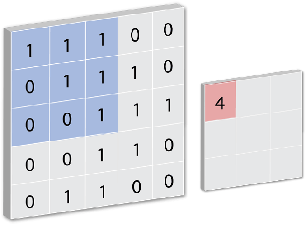 CREDIT: FLETCHER BACH[/caption]
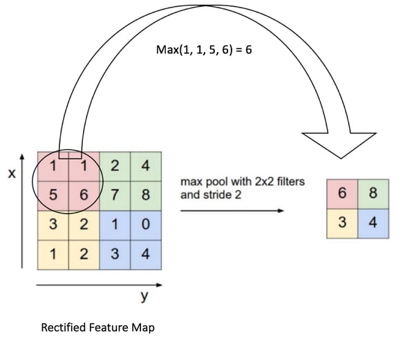
What is MaxPooling2D?
A MaxPooling2D layer is often used after a CNN layer in order to reduce the complexity of the output and prevent overfitting of the data. In this case we chose a size of two. This means the size of the output matrix of this layer is only half of the input matrix.
 With that out of the way, let’s continue and see the architecture of our model.
model.summary()

 _________________________________________________________________
 Layer (type) Output Shape Param #
 =================================================================
 conv2d_1 (Conv2D) (None, 26, 26, 32) 320
 _________________________________________________________________
 max_pooling2d_1 (MaxPooling2 (None, 13, 13, 32) 0
 _________________________________________________________________
 conv2d_2 (Conv2D) (None, 11, 11, 64) 18496
 _________________________________________________________________
 max_pooling2d_2 (MaxPooling2 (None, 5, 5, 64) 0
 _________________________________________________________________
 conv2d_3 (Conv2D) (None, 3, 3, 64) 36928
 =================================================================
 Total params: 55,744 Trainable params: 55,744 Non-trainable params: 0
 _________________________________________________________________
As you can see, the output of each Conv2D and MaxPooling2D is a 3D tensor of shape (height, width, channel). The height and width parameters lower as we progress through our network. We will take the last output tensor of shape (3,3,64) and feed it to a densely connected classifier network. Keep in mind classifiers process the 1D vectors, so we have to flatten our 3D vector to 1D vector. Also, since we are classifying 10 digits (0–9), we need a 10-way classifier with a softmax activation. Let’s do that.
model.add(layers.Flatten())
 model.add(layers.Dense(64, activation='relu'))
 model.add(layers.Dense(10, activation='softmax'))
Let’s quickly print our model architecture again.
model.summary()

 Layer (type) Output Shape Param #
 =================================================================
 conv2d_1 (Conv2D) (None, 26, 26, 32) 320
 _________________________________________________________________
 max_pooling2d_1 (MaxPooling2 (None, 13, 13, 32) 0
 _________________________________________________________________
 conv2d_2 (Conv2D) (None, 11, 11, 64) 18496
 _________________________________________________________________
 max_pooling2d_2 (MaxPooling2 (None, 5, 5, 64) 0
 _________________________________________________________________
 conv2d_3 (Conv2D) (None, 3, 3, 64) 36928
 _________________________________________________________________
 flatten_1 (Flatten) (None, 576) 0
 _________________________________________________________________
 dense_1 (Dense) (None, 64) 36928
 _________________________________________________________________
 dense_2 (Dense) (None, 10) 650
 =================================================================
 Total params: 93,322 Trainable params: 93,322 Non-trainable params: 0
As you can see from above (3,3,64) outputs are flattened into vectors of shape (,576) (i.e. 3x3x64= 576) before feeding into dense layers.
Step 2: Train the model
Let’s train our model. The mnist dataset is split into train and test samples of 60k and 10k respectively.
from keras.datasets import mnist
 from keras.utils import to_categorical

  (train_images, train_labels), (test_images, test_labels) = mnist.load_data()

 train_images = train_images.reshape((60000, 28, 28, 1))
 train_images = train_images.astype('float32') / 255

 test_images = test_images.reshape((10000, 28, 28, 1))
 test_images = test_images.astype('float32') / 255

 train_labels = to_categorical(train_labels)
 test_labels = to_categorical(test_labels)

 model.compile(optimizer='rmsprop',
  loss='categorical_crossentropy',
  metrics=['accuracy'])
 model.fit(train_images, train_labels, epochs=5, batch_size=64)
Step 3: Evaluate the model against test dataset
We use model.evaluate() and pass in the test_images and test_labels that we created in the previous step. This function will calculate loss and accuracy on the test data set.
test_loss, test_acc = model.evaluate(test_images, test_labels)
Let’s check the accuracy.
test_acc
 0.9914
Finally we test the accuracy of our model on the test dataset — it's about 99.14 percent accurate! Not a bad start! Please note your numbers might slightly differ based on various factors when you actually run this code.
Summary
We have trained and evaluated a simple image classifier CNN model with Keras. I have made the full code available
here on github. Feel free to download and experiment with it; try to train your model by changing various parameters such as number of epochs, layers and a different loss function etc. As always, happy learning :)
Note: This was originally posted on
Medium.

