Apache Cassandra promises linear scalability and workload distribution, among many other features—and rightly so. However, as with many good things in life, these benefits come with a set of upfront conditions.

When the use case aligns with the architectural limitations, Cassandra excels at storing and accessing datasets up to petabytes in volume, delivering impressive throughput. As the data or workload volume grows, we expand the cluster linearly, ensuring consistent performance.

However, even when we adhere to the documentation and best practices and create an effective data model, we might encounter underperforming nodes or unexpected challenges with throughput scaling after a cluster expansion—and it’s not always clear what causes the imbalance. Linear scalability relies on the assumption that workload and data are evenly distributed across all nodes in a cluster, and the cluster capacity relates directly to the number of nodes. Sometimes, these conditions aren’t met, affecting linear scalability. So, we strive for scalability and balance and are willing to fulfill the necessary conditions.

However, this can prove challenging since there isn’t any comprehensive documentation on Cassandra’s scalability and balance compromises and how to address them. Additionally, the causes mentioned in this post come from real experiences in production systems, with some being common pain points.

The goal of this post is to shed light on Cassandra’s scalability compromises. Though it won’t cover everything that can go wrong, it will focus on the most common desk-flipping causes of poor scalability.

Poor scalability, as in…?

Before delving into the details, it’s important to clarify the problem this post aims to help you solve or prevent. To that end, here’s a definition of poor scalability in the context of this blog post:

Poor Scalability: This occurs in a Cassandra cluster when either data or workload distributions have high variance across all nodes, often associated with systematic hardware-bound bottlenecks in a node or subset of nodes. It inevitably results in cases where performance doesn’t scale linearly with node addition and/or removal.

With the scope of the problem now clarified, let’s explore the conditions that may lead to its manifestation.

Virtual token generation

Before diving in, let’s briefly discuss the history of virtual nodes.

To understand virtual nodes, we must first grasp what Cassandra tokens are. Tokens are integer numbers ranging from -(2^63) to (2^63)-1. This range of sequential integers represents a Cassandra token ring (imagine a bagel composed of 2^64 radial slices), where -2^63 is the next value after 2^63-1, closing the ring.

In the initial releases, each Cassandra node owned exactly one primary token. A token range includes every value between two primary tokens in sequence. This method is useful because partition key values are hashed into token values to better distribute them across Cassandra nodes.

In version 1.2, Apache Cassandra introduced a new feature—virtual tokens.

This feature primarily aimed to simplify cluster scaling. Previously, it was necessary to manually calculate and define a single token per node—an easy task until keeping your cluster load balanced required expanding beyond the desired capacity.

For example, consider a cluster with three nodes, splitting the full range of tokens into three equally sized sub-ranges. To expand while keeping all nodes balanced, you’d have to add at least three more nodes. Want to scale up again? You need to expand by a multiple of three. Want the actual token sub-ranges to have a fixed size? You’d need exponential expansion. This rationale also applies to scaling down.

This inflexible approach to scalability not only limited the “right” number of replicas but also added complexity to managing and defining tokens for new nodes. Enter virtual nodes designed to resolve these limitations.

Representing the problem of balanced expansion in a cluster with single tokens:

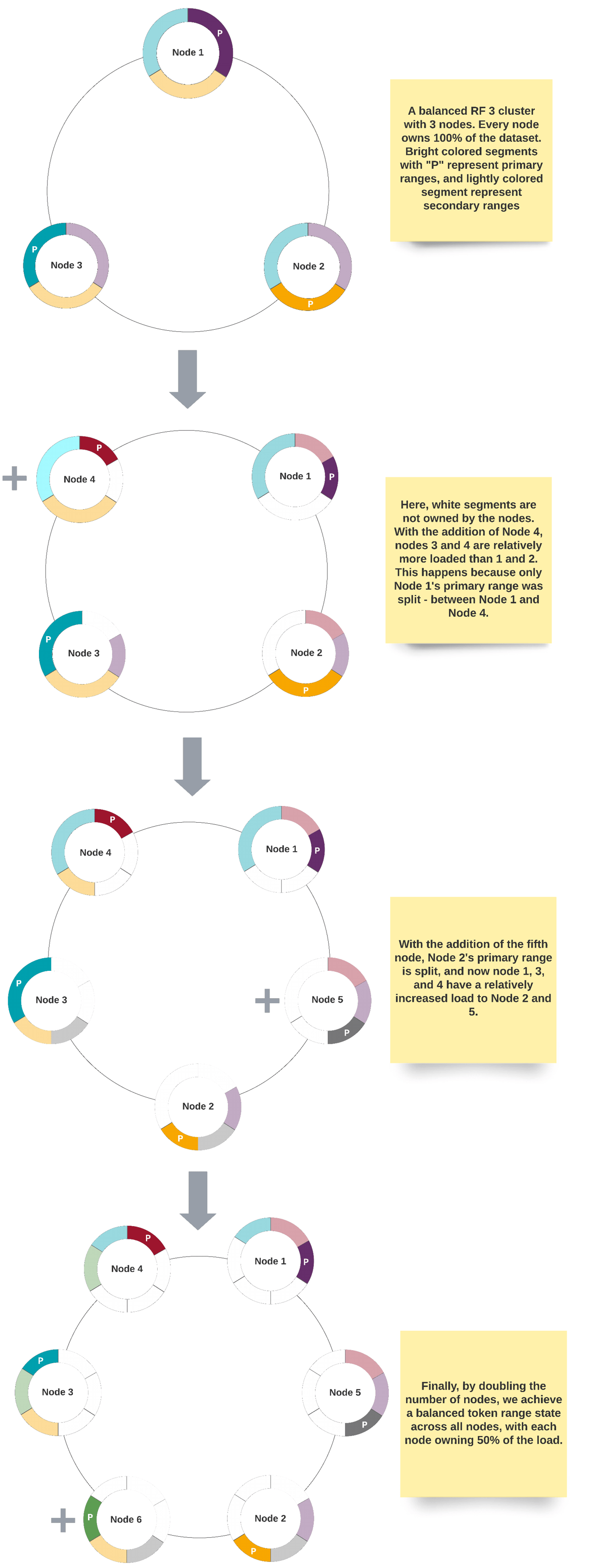
With virtual nodes, each Cassandra node represents a fixed number of virtual nodes, and each virtual node owns a primary token. This approach partially solves the problem of flexible scaling while maintaining balance by spreading the range of tokens across randomly sized virtual token ranges. Additionally, Cassandra users no longer need to plan and specify tokens when adding nodes—Cassandra handles that automatically. While this may sound promising, there are still some challenges to consider.

Randomness in token generation

The virtual tokens are generated randomly, which means that there’s no guarantee the dataset will be split evenly. While you can still manually declare the tokens, you’d have to calculate and manage a balancing act for multiple primary tokens per Cassandra node instead of just one token per node. As a result, users seeking to capitalize on the ease of adding nodes with virtual nodes often rely on the random token generator rather than manual configuration.

The solution for the token range variance generated by random token generation was to set the virtual node cardinality to 256, which remained the default until the latest Apache Cassandra 3.X versions. With 256 virtual nodes, even though the token range size variance exists due to randomness, the variance is diluted across a high number of virtual nodes per node, mitigating the variance at the Cassandra node level. While this may seem promising, it’s still not an ideal solution.

Performance and availability impact

While using 256 virtual nodes somewhat addressed the problem of dataset distribution, it introduced a new set of challenges. The increase in virtual nodes made cluster-wide operations, such as anti-entropy repairs, more expensive (i.e., less scalable) and reduced availability. With greater granularity in token ranges, the likelihood of LOCAL_QUORUM requests failing (with a replication factor of 3) increased when two nodes were down in a data center. To better understand how availability is affected, consider the following image representing the scenario with and without virtual nodes:

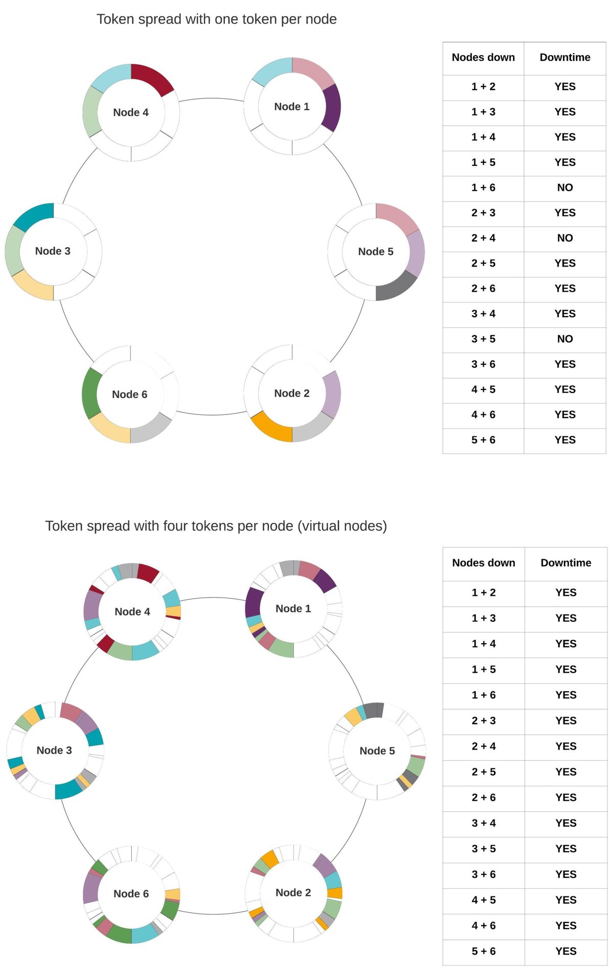
If two nodes are down and share at least one colored shape, it means that the corresponding token range is not available for writes or reads with QUORUM. In both presented scenarios, the replication strategy is SimpleStrategy. Using NetworkTopologyStrategy instead, we can increase availability, as any number of nodes within a single rack can be unavailable without affecting QUORUM requests when the replication is at least three and nodes are split across three or more racks.

From the example, it’s evident that with virtual nodes, as token ranges are dispersed more granularly, the chances of downtime are higher when two nodes are down. Another aspect to take away from this example is that since tokens are randomly generated, and the replication logic doesn’t attempt to replicate around data load but rather around token sequence, we can observe high variance in token ownership across nodes (note Node 1 vs. Node 5).

 

With this newfound knowledge, there was an urge to find a good balance between a high enough number of virtual nodes to distribute data evenly and low enough to minimize performance and availability compromises. Generally speaking, 16 to 32 virtual nodes can achieve an acceptable amount of token ownership variance if you’re using the default random token generation algorithm. But we can go lower than 16. I’ll explain how next.

How to deploy a balanced cluster with only 4 virtual nodes

If you are deploying a new cluster with more than 3 nodes in Apache Cassandra 3.0 or later, it’s simple to start this.

First, you specify a low number of virtual nodes in cassandra.yaml. This needs to be applied consistently to every node in the logical data center:

num_tokens: 4

Next, you deploy the first 3 nodes (assuming a replication factor of 3) normally.

Then you change the native keyspaces’ system_distributed, system_traces and system_auth replication strategy to match your production keyspace (more about the whys and hows here):

ALTER KEYSPACE system_distributed WITH replication = {'class': 'NetworkTopologyStrategy', '<datacenter_name>': 3 };

ALTER KEYSPACE system_traces WITH replication = {'class': 'NetworkTopologyStrategy', '<datacenter_name>': 3 };

ALTER KEYSPACE system_auth WITH replication = {'class': 'NetworkTopologyStrategy', '<datacenter_name>': 3 };

After adding the first three nodes and changing replication strategies for native keyspaces, you still specify the same num_tokens parameter for every additional node before bootstrapping, along with an additional parameter in cassandra.yaml:

allocate_tokens_for_keyspace: system_traces

Even though you shouldn’t have any data in this keyspace, the replication logic is consistent for all keyspaces using the same strategy. Based on that, Cassandra will calculate tokens based on the current logical distribution of tokens in the cluster in an attempt to decrease token ownership variance, as opposed to the default random token generation that would leave balance at the mercy of four 2^64-sized dice rolls.

This allocation strategy is also valid for cluster expansions. You can’t change the tokens of a node once it bootstraps, but you can (and should) define the token generation of new nodes using allocate_tokens_for_keyspace, which indirectly affects the general balance of a cluster – in the case of DataStax Enterprise, use allocate_tokens_for_replication_factor: <RF_number_here>.

It must be said that this is only effective when all populated keyspaces share the same replication strategy and, depending on the Cassandra version, the partitioner is Murmur3Partitioner.

Partition hotspots

We’ll now move away from token imbalance and focus on scalability tied to data model design, starting with partition design.

As with most data stores, in Cassandra, data modeling is crucial to ensure good database performance. Specifically in Cassandra because each table is designed to satisfy one application query and can’t be easily changed at the partition level without requiring data migrations between tables or adding complexity at the application level.

For this reason, it’s essential to identify application query patterns beforehand and design Cassandra tables accordingly. But even that may not be enough.
Because data is distributed across Cassandra nodes in partition units, uneven partitions can result in data imbalance. This can manifest at many levels:

• Dataset growth scales up partition size more so than partition cardinality
• Query activity is heavily focused on a small subset of partitions
• Oddly distributed large partitions in the dataset (>100MB)

All of the factors above result from suboptimal data modeling, and can only be fully addressed at a data model level. This is one of the many reasons we recommend seeking a Cassandra SME to help design a scalable and performant data model before deploying a Cassandra cluster supporting Production services. If a deployed Cassandra cluster is planned to scale up in size with the underlying service(s), and the data model doesn’t accommodate scalability, the costs of addressing this issue will only increase over time.

Partition hotspots: an example

Let’s bring back the 6-node cluster from the previous examples and see how large partitions could affect data distribution. More precisely, we’re going to see an example of variance in the average partition size per token range that can affect data distribution. I named each token range from A through F to help track impact at the node level. So we have a balanced cluster token-wise:

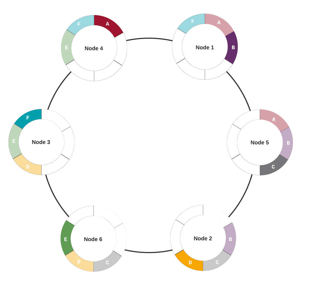
Looks good so far. For the sake of deeper analysis, I’ll design an arbitrary example with large partitions and some (exaggerated) variance in average partition size using the setup above:

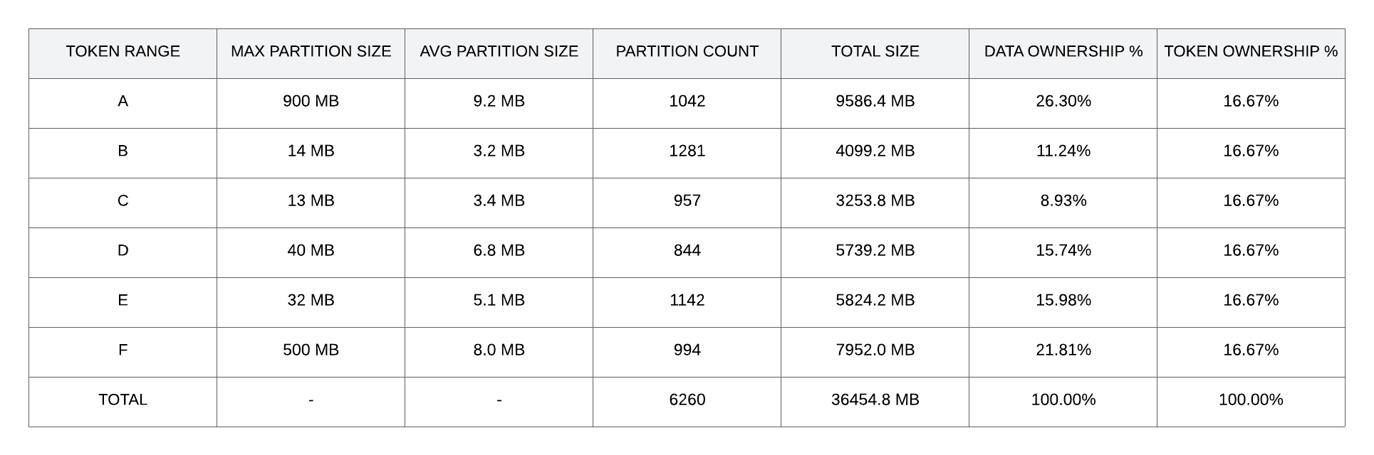
Doesn’t look so great now. There are two ranges with partitions over 100 MB, which tends to be a rule-of-thumb threshold to watch for regarding read latencies. Moreover, the partition count is balanced, this is generally expected, as the Murmur3Partitioner does a pretty good job at distributing the load across the token ring, and all of the token ranges here are perfectly balanced in the token count.

However, the average partition size is far from balanced across these token ranges, and consequently, the dataset split among the token ranges is also imbalanced. A good way to measure this effect is to compare the percentages of data and token ownership on the rightmost columns. Ideally, we want both as close as possible, which they’re not in this example. Let’s see how this would affect real load at the node level:

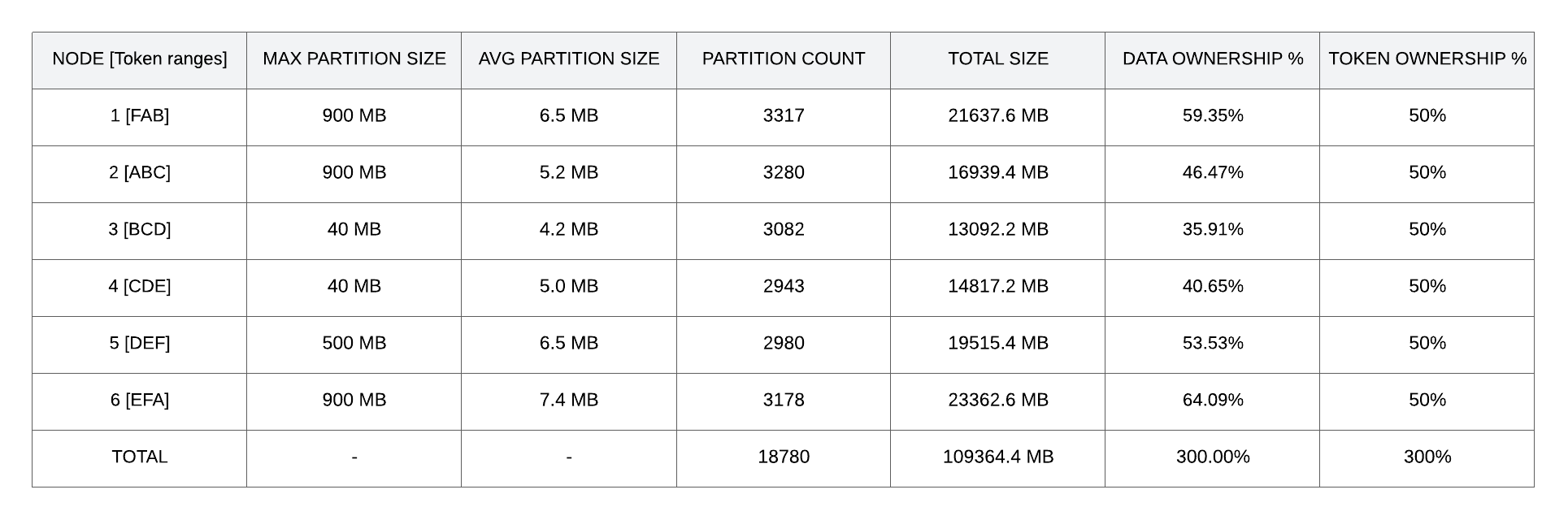
In this last table, we can measure the effect of the suboptimal conditions set in the previous table at the node level. I’d like to reiterate that this is a perfectly balanced cluster token-wise, where each node owns 50% of the tokens, as represented in the cluster image. Large partitions lead to an increase in data load in some ranges, and therefore nodes are also imbalanced. Here we can measure imbalance by comparing data ownership percentages between the nodes. In this case, we can see that node 6 has almost doubled its load relative to node 3, and most nodes stray far from the ideal 50%.

Generally, balancing tokens is the best way to deal with data imbalance. Still, in situations analogous to this example, the problem has to be addressed at the data model level since data imbalance is directly related to partition size distribution.
In other words, if we can visualize all partitions by ascending order of size, we want the growth line to be as linear and flat as possible to guarantee a matching balance with the token ring.

Partition distribution

Even when you get size distribution across partitions right, partitions can be poorly distributed across the cluster. This can happen due to poor token distribution, as described above in the Virtual Token Generation section, but can also be tied to partitioner hashing.

Cassandra partitioners consistently convert every partition key to a hash value that, in turn, translates to a token value. The hashing function tries to be as random as possible to distribute partitions indiscriminately across all replicas. The more partitions a table has, the less likely it is that they are unevenly distributed. However, if the number of partitions doesn’t exceed the number of nodes by more than 1 order of magnitude, the likelihood of getting undistributed partitions becomes concerning.

In the following representation, I aim to present what can be considered poor distribution due to a low partition count to node count ratio.

 

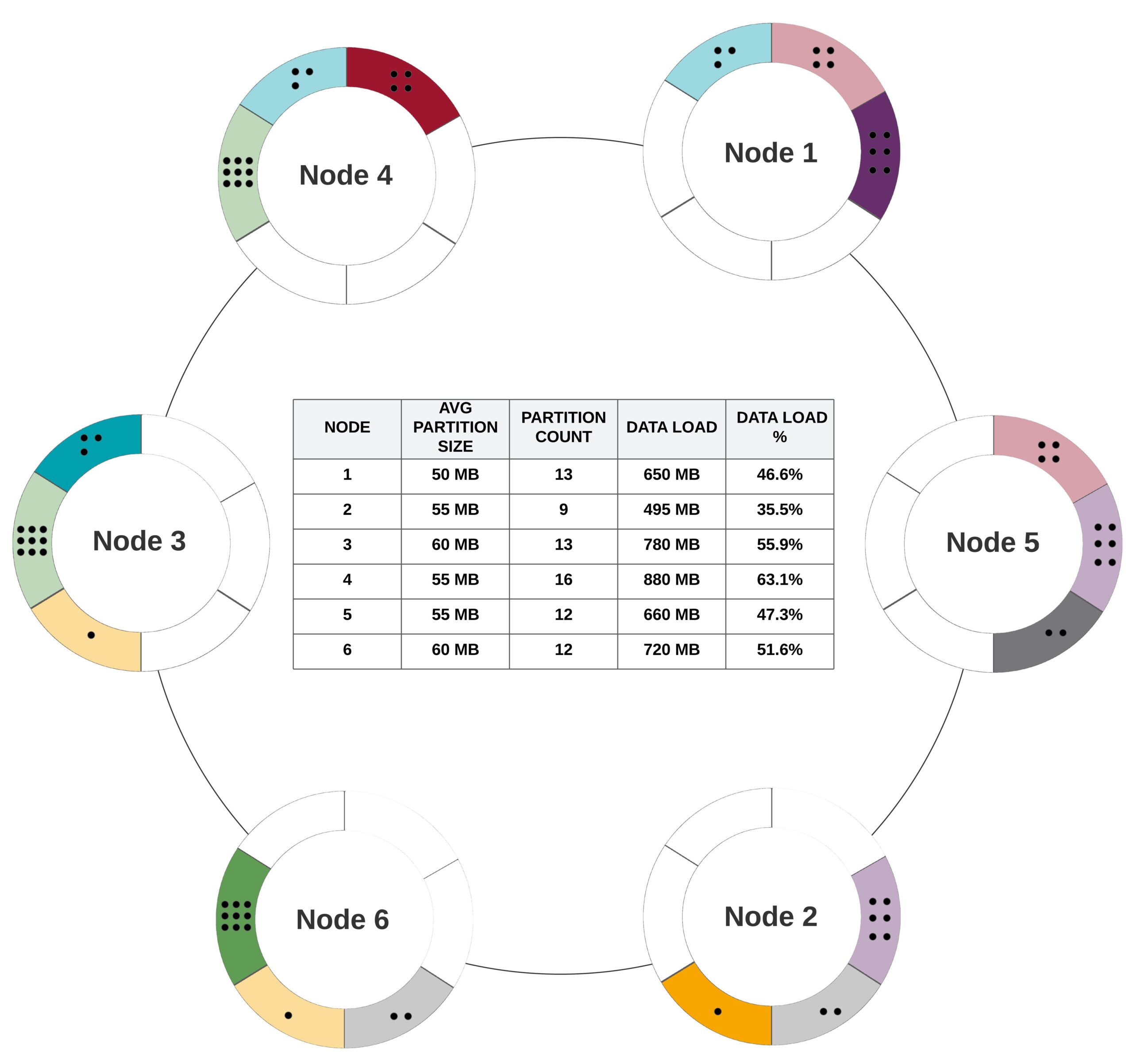
In this representation, each dot represents a partition table with a relatively small dataset. There are 25 partitions spread across six primary tokens and six nodes.

Given the small partition cardinality to token cardinality ratio, having high variance in partition per range is a likely scenario. Consider 25 independent classic dice rolls to allocate each partition to one of 6 ranges. In order to minimize variance in distribution we want more dice rolls and/or less faces on the dice (i.e., more partitions and/or fewer nodes). The imbalance results in high variance in load. This is especially impactful when you have a read-heavy workload running against a table with low partition cardinality. In this example, it’s expected from node 4 to do nearly double the work of node 2 against the existing partitions in the table. As with hotspots, it can be a data modelling pitfall and should be avoided at all costs.

Secondary Indexes

In Cassandra, secondary indexes populate hidden tables that dynamically track the indexed column value. This column effectively serves as a partition key in the hidden table, while the primary key values from the base table function as clustering columns. When you read from a secondary index in Cassandra, you’re actually reading from two tables–first, the secondary index table and then the base table for each secondary index row. A single secondary index read often triggers multiple internal reads in the base table.

In the case of low-cardinality indexes, secondary index “partitions” can become extremely large, affecting read performance more than scalability. When heavily read indexed values are replicated across only a small subset of partitions, balance can be impacted, as the same subset of replicas has to deal with the overhead of Cassandra secondary indexes repeatedly. If nothing breaks in the process, consider yourself fortunate.

With high-cardinality indexes, the main issue is wasting cycles requesting data from replicas that don’t actually own it. While this problem is more manageable regarding Cassandra performance compared to low-cardinality indexes, it’s arguably more impactful at the scalability level. The number of replicas not owning the data for each request scales with cluster size, along with coordinator work.

Cassandra’s secondary indexes seldom perform at scale and only do so in a limited range of scenarios. To adequately cover this topic, an entire blog post would be necessary.

In summary, when it comes to secondary indexes, if you don’t truly need them, don’t use them. If you think you need them, consult a Cassandra Subject Matter Expert (SME)–there are likely better ways to achieve your goals within or outside of Cassandra. If you do choose to use secondary indexes, do so sparingly.

Aggregation Queries

Ah, yes, aggregation queries…one of my pet peeves in Cassandra workloads. Before I explain why they are an absolute don’t, let me define what they are:

Aggregation query: Any non-secondary index SELECT query where you’re not searching by partition key value, commonly (but not necessarily) containing ALLOW_FILTERING. This includes queries using native aggregate functions (i.e., COUNT, MAX, MIN, SUM, and AVG).

When performing this type of query, Cassandra reads all the data in a table, or at least all the data, until a specified LIMIT of results is reached for each replica. Add the filtering overhead to this, and consider that the data you seek is not indexed for your query. Additionally, this work is executed on at least 1/RF (Replication Factor) of your nodes, multiplied by the consistency level. Lastly, consider the increased chance of read repairs blocking requests on multiple replica sets. Saying this is bad for your database’s health is an understatement. It may not break your cluster, but it could, depending on the read size and concurrent operations.

Obviously, indiscriminately reading all data, possibly from a third up to the cluster’s totality, doesn’t scale well, even with limited results. Using limits helps avoid a full dataset scan, but Cassandra still runs the query on a fixed fraction of nodes, meaning costs scale up with cluster size. This query type can be used sparingly but is not scalable if relied upon heavily.

This raises the question: “If it’s so bad, why is it available? Are there any alternatives?”

Aggregate queries exist for flexibility of use and testing purposes, but they also bypass the foundational principles of Cassandra architecture. Similarly, one can bypass traffic lights while driving, but this puts themself, other drivers, and bystanders at risk and likely negatively affects the road system’s throughput.

As for alternatives, beyond splitting queries across denormalized tables or using secondary indexes, Cassandra doesn’t provide much query flexibility for non-partition reads. Joins are unavailable and must be managed at the application level if absolutely necessary. Querying by non-partition columns is possible via secondary indexes but should be used cautiously for several reasons, some of which were explained in the previous section.

Conclusion

Poor scalability can result from several causes, but it is commonly related to suboptimal token distribution, data model anti-patterns, or unscalable queries. Out of these three, token distribution is the easiest to address if you’re using Apache Cassandra 3+ by expanding the cluster with a logical token generator, as opposed to the default random one.

Partition cardinality and size are also important. Scalability and/or cluster balance decrease in relation to the combination of low cardinality and high variance in partition size.

If a service heavily relies on Cassandra secondary indexes or aggregation queries, it must be accepted that this comes at the cost of lower performance and scalability.

There are other causes not addressed here, such as imbalance at the logical topology level or dynamic snitch misconfiguration, but these tend to be more niche cases and, in some ways, are easier to address.